Tutorial 4: Protein DMS modeling using a biophysical G-P map
[1]:
# Standard imports
import numpy as np
import pandas as pd
import matplotlib.pyplot as plt

# Special imports
import mavenn
Here we show how to train and visualize a thermodynamic model describing the folding and IgG-binding of protein GB1 variants. This model was first proposed by Otwinowski (2018), who trained it on the DMS data of Olson et al. (2014). Here we repeat this exercise within the MAVE-NN framework, thus obtaining a model similar to the one featured in Figs. 6a and 6b of Tareen et al. (2021). The mathematical form of this G-P map is explianed in the supplemental material of Tareen et al. (2021); see in particular Fig. S4a.
Defining a custom G-P map
First we define a custom G-P map that represents our biophysical model. We do this by subclassing CustomGPMapLayer to get a custom G-P map class called OtwinowskiGPMapLayer. This subclassing procedure requires that we fill in the bodies of two specific methods.
__init__(): This constructor must first call the superclass constructor, which sets the attributesL,C, andregularizer. The the derived class constructor then defines all of the trainable parameters of the G-P map:theta_f_0,theta_b_0,theta_f_lc, andtheta_b_lcin this case.call(): This is the meat of the custom G-P map. The inputx_lcis a one-hot encoding of all sequences in a minimatch. It has size[-1, L, C], where the first index runs over minibatch examples. The G-P map parameters are then used to compute and return a vectorphiof latent phenotype values, one for each input sequence in the minibatch.
[2]:
# Standard TensorFlow imports
import tensorflow as tf
import tensorflow.keras.backend as K
from tensorflow.keras.initializers import Constant

# Import base class
from mavenn.src.layers.gpmap import GPMapLayer

# Define custom G-P map layer
class OtwinowskiGPMapLayer(GPMapLayer):
    """
    A G-P map representing the thermodynamic model described by
    Otwinowski (2018).
    """

    def __init__(self, *args, **kwargs):
        """Construct layer instance."""

        # Call superclass constructor
        # Sets self.L, self.C, and self.regularizer
        super().__init__(*args, **kwargs)

        # Initialize constant parameter for folding energy
        self.theta_f_0 = self.add_weight(name='theta_f_0',
                                         shape=(1,),
                                         trainable=True,
                                         regularizer=self.regularizer)

        # Initialize constant parameter for binding energy
        self.theta_b_0 = self.add_weight(name='theta_b_0',
                                         shape=(1,),
                                         trainable=True,
                                         regularizer=self.regularizer)

        # Initialize additive parameter for folding energy
        self.theta_f_lc = self.add_weight(name='theta_f_lc',
                                          shape=(1, self.L, self.C),
                                          trainable=True,
                                          regularizer=self.regularizer)

        # Initialize additive parameter for binding energy
        self.theta_b_lc = self.add_weight(name='theta_b_lc',
                                          shape=(1, self.L, self.C),
                                          trainable=True,
                                          regularizer=self.regularizer)

    def call(self, x_lc):
        """Compute phi given x."""

        # 1kT = 0.582 kcal/mol at room temperature
        kT = 0.582

        # Reshape input to samples x length x characters
        x_lc = tf.reshape(x_lc, [-1, self.L, self.C])

        # Compute Delta G for binding
        Delta_G_b = self.theta_b_0 + \
                    tf.reshape(K.sum(self.theta_b_lc * x_lc, axis=[1, 2]),
                               shape=[-1, 1])

        # Compute Delta G for folding
        Delta_G_f = self.theta_f_0 + \
                    tf.reshape(K.sum(self.theta_f_lc * x_lc, axis=[1, 2]),
                               shape=[-1, 1])

        # Compute and return fraction folded and bound
        Z = 1+K.exp(-Delta_G_f/kT)+K.exp(-(Delta_G_f+Delta_G_b)/kT)
        p_bf = (K.exp(-(Delta_G_f+Delta_G_b)/kT))/Z
        phi = p_bf #K.log(p_bf)/np.log(2)
        return phi
Training a model with a custom G-P map
Next we load the 'gb1' dataset, compute sequence length, and split the data into a test set and a training+validation set.
[3]:
# Choose dataset
data_name = 'gb1'
print(f"Loading dataset '{data_name}' ")

# Load datset
data_df = mavenn.load_example_dataset(data_name)

# Get and report sequence length
L = len(data_df.loc[0,'x'])
print(f'Sequence length: {L:d} amino acids')

# Split dataset
trainval_df, test_df = mavenn.split_dataset(data_df)

# Preview trainval_df
print('trainval_df:')
trainval_df
Loading dataset 'gb1'
Sequence length: 55 amino acids
Training set   :  477,854 observations (  90.04%)
Validation set :   26,519 observations (   5.00%)
Test set       :   26,364 observations (   4.97%)
-------------------------------------------------
Total dataset  :  530,737 observations ( 100.00%)

trainval_df:
[3]:
| validation | dist | input_ct | selected_ct | y | x | |
|---|---|---|---|---|---|---|
| 0 | False | 2 | 173 | 33 | -3.145154 | AAKLILNGKTLKGETTTEAVDAATAEKVFKQYANDNGVDGEWTYDD... |
| 1 | False | 2 | 18 | 8 | -1.867676 | ACKLILNGKTLKGETTTEAVDAATAEKVFKQYANDNGVDGEWTYDD... |
| 2 | False | 2 | 66 | 2 | -5.270800 | ADKLILNGKTLKGETTTEAVDAATAEKVFKQYANDNGVDGEWTYDD... |
| 3 | False | 2 | 72 | 1 | -5.979498 | AEKLILNGKTLKGETTTEAVDAATAEKVFKQYANDNGVDGEWTYDD... |
| 4 | False | 2 | 69 | 168 | 0.481923 | AFKLILNGKTLKGETTTEAVDAATAEKVFKQYANDNGVDGEWTYDD... |
| ... | ... | ... | ... | ... | ... | ... |
| 504368 | False | 2 | 462 | 139 | -2.515259 | QYKLILNGKTLKGETTTEAVDAATAEKVFKQYANDNGVDGEWTYDD... |
| 504369 | False | 2 | 317 | 84 | -2.693165 | QYKLILNGKTLKGETTTEAVDAATAEKVFKQYANDNGVDGEWTYDD... |
| 504370 | False | 2 | 335 | 77 | -2.896589 | QYKLILNGKTLKGETTTEAVDAATAEKVFKQYANDNGVDGEWTYDD... |
| 504371 | False | 2 | 148 | 28 | -3.150861 | QYKLILNGKTLKGETTTEAVDAATAEKVFKQYANDNGVDGEWTYDD... |
| 504372 | False | 2 | 95 | 16 | -3.287173 | QYKLILNGKTLKGETTTEAVDAATAEKVFKQYANDNGVDGEWTYDD... |
504373 rows × 6 columns
Next we create an instance of the mavenn.Model class. In addition to standard keyword arguments for GE regression, we pass keyword arguments specific to the use of our custom G-P map:
gpmap_type='custom': Alerts themavenn.Model()constructor that we wish to use a custom G-P map.custom_gpmap=OtwinowskiGPMapLayer: Specifies the specific class to use for the custom G-P map layer.gpmap_kwargs=gpmap_kwargs: Provides a dictionary of arguments to be passed to the constructor of the custom G-P map.
[4]:
# Order the alphabet to match Otwinowski (2018)
alphabet = np.array(list('KRHEDNQTSCGAVLIMPYFW'))
C = len(alphabet)

# define custom gp_map parameters dictionary
gpmap_kwargs = {'L':L,
                'C':C,
                'theta_regularization': 0.0005}

# Create model instance
model = mavenn.Model(L=L,
                     alphabet=alphabet,
                     regression_type='GE',
                     ge_nonlinearity_type='nonlinear',
                     ge_nonlinearity_monotonic=False,
                     ge_noise_model_type='SkewedT',
                     ge_heteroskedasticity_order=2,
                     ge_nonlinearity_hidden_nodes=100,
                     eta_regularization=0.0001,
                     gpmap_type='custom',
                     normalize_phi=False,
                     custom_gpmap=OtwinowskiGPMapLayer,
                     gpmap_kwargs=gpmap_kwargs)
As in previous tutorials, we then set the training data using model.set_data() and then train the model using model.fit().
[5]:
# Set False->True to train model
if True:

    # Set training data
    model.set_data(x=trainval_df['x'],
                   y=trainval_df['y'],
                   validation_flags=trainval_df['validation'])

    # Train model
    model.fit(learning_rate=.0005,
              epochs=1000,
              batch_size=300,
              early_stopping=True,
              early_stopping_patience=50,
              linear_initialization=False,
              verbose=False)

    # Save model to file
    model_name = f'{data_name}_thermodynamic_model'
    model.save(model_name)
N = 504,373 observations set as training data.
Using 5.3% for validation.
Data shuffled.
Time to set data: 8.71 sec.
Training time: 1062.1 seconds
Model saved to these files:
        gb1_thermodynamic_model.pickle
        gb1_thermodynamic_model.weights.h5
Next we evaluate the performance of the model on test data and save the model to disk.
Visualizing models with custom G-P maps
One can load the custom G-P map model and analyze its training history / performance in the same way as with built-in G-P map, e.g.:
[6]:
# Load model from file
model_name = f'{data_name}_thermodynamic_model'
model = mavenn.load(model_name)

# Compute variational information on test data
I_var, dI_var =  model.I_variational(x=test_df['x'], y=test_df['y'])
print(f'test_I_var: {I_var:.3f} +- {dI_var:.3f} bits')

# Compute predictive information on test data
I_pred, dI_pred = model.I_predictive(x=test_df['x'], y=test_df['y'])
print(f'test_I_pred: {I_pred:.3f} +- {dI_pred:.3f} bits')
Model loaded from these files:
        gb1_thermodynamic_model.pickle
        gb1_thermodynamic_model.weights.h5
test_I_var: 2.320 +- 0.015 bits
test_I_pred: 2.355 +- 0.008 bits
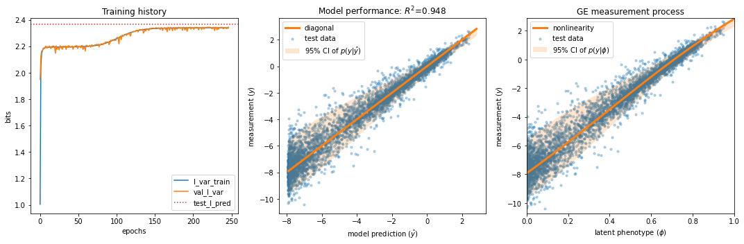
[7]:
# Get quantities to plot
y_test = test_df['y']
N_test = len(y_test)
yhat_test = model.x_to_yhat(test_df['x'])
phi_test = model.x_to_phi(test_df['x'])
phi_lim = [0, 1]
phi_grid = np.linspace(phi_lim[0], phi_lim[1], 1000)
yhat_grid = model.phi_to_yhat(phi_grid)
q = [0.025, 0.975]
yqs_grid = model.yhat_to_yq(yhat_grid, q=q)
ix = np.random.choice(a=N_test, size=5000, replace=False)
Rsq = np.corrcoef(yhat_test.ravel(), test_df['y'])[0, 1]**2

# Create figure and axes for plotting
fig, axs = plt.subplots(1,3,figsize=[15,5])

# Plot panel 1: Training history
ax = axs[0]
ax.plot(model.history['I_var'],
        label=r'I_var_train')
ax.plot(model.history['val_I_var'],
        label=r'val_I_var')
ax.axhline(I_pred, color='C3', linestyle=':',
           label=r'test_I_pred')
ax.set_xlabel(r'epochs')
ax.set_ylabel(r'bits')
ax.set_title(r'Training history')
ax.legend()

## Panel 2: R^2 model performance
ax = axs[1]
ax.scatter(yhat_test[ix], y_test[ix], color='C0', s=10, alpha=.3,
           label=r'test data')
#xlim = [min(yhat_test), max(yhat_test)]
#ax.plot(xlim, xlim, '--', color='k', label='diagonal', zorder=100)
ax.fill_between(yhat_grid, yqs_grid[:, 0], yqs_grid[:, 1],
                alpha=0.2, color='C1', lw=0, label=r'95% CI of $p(y|\hat{y})$')
ax.plot(yhat_grid, yhat_grid,
        linewidth=3, color='C1', label='diagonal')
ax.set_xlabel(r'model prediction ($\hat{y}$)')
ax.set_ylabel(r'measurement ($y$)')
ax.set_title(rf'Model performance: $R^2$={Rsq:.3}');
ax.legend()

## Panel 3: GE plot
ax = axs[2]
ax.scatter(phi_test[ix], y_test[ix],
           color='C0', s=10, alpha=.3, label=r'test data')
ax.fill_between(phi_grid, yqs_grid[:, 0], yqs_grid[:, 1],
                alpha=0.2, color='C1', lw=0, label=r'95% CI of $p(y|\phi)$')
ax.plot(phi_grid, yhat_grid,
        linewidth=3, color='C1', label=r'nonlinearity')
ax.set_ylim([min(y_test), max(y_test)])
ax.set_xlim(phi_lim)
ax.set_xlabel(r'latent phenotype ($\phi$)')
ax.set_ylabel(r'measurement ($y$)')
ax.set_title(r'GE measurement process')
ax.legend()
fig.tight_layout()
To retrieve the parameters of our custom G-P map, we again use the method model.get_theta(). This returns the dictionary provided by our custom G-P map via the method get_params():
[8]:
# Retrieve G-P map parameter dict and view dict keys
theta_dict = model.layer_gpmap.get_params()
theta_dict.keys()
[8]:
dict_keys(['theta_f_0', 'theta_b_0', 'theta_f_lc', 'theta_b_lc'])
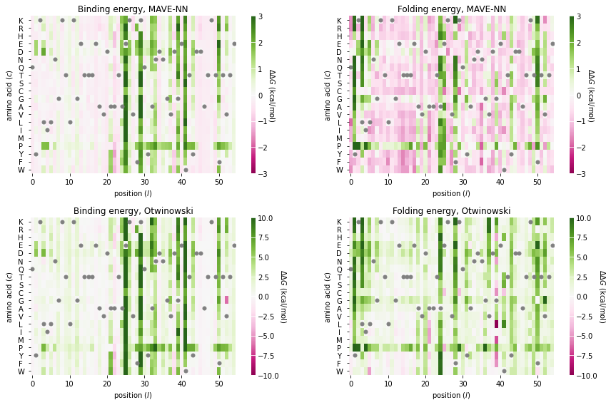
Next we visualize the additive parameters that determine both folding energy(theta_b_lc) and binding energy (theta_r_lc). Note that we visualize these as parameters as changes (ddG_f and ddG_b) with respect to the wild-type sequence. It is also worth comparing these \(\Delta \Delta G\) values to those inferred by Otwinowski (2019).
[9]:
# Get the wild-type GB1 sequence
wt_seq = model.x_stats['consensus_seq']

# Convert this to a one-hot encoded matrix of size LxC
from mavenn.src.utils import _x_to_mat
x_lc_wt = _x_to_mat(wt_seq, model.alphabet)

# Subtract wild-type character value from parameters at each position
ddG_b_mat_mavenn = theta_dict['theta_b_lc'] - np.sum(x_lc_wt*theta_dict['theta_b_lc'], axis=1)[:,np.newaxis]
ddG_f_mat_mavenn = theta_dict['theta_f_lc'] - np.sum(x_lc_wt*theta_dict['theta_f_lc'], axis=1)[:,np.newaxis]

# Load Otwinowski parameters form file
dG_b_otwinowski_df = pd.read_csv('../../mavenn/examples/datasets/raw/otwinowski_gb_data.csv.gz', index_col=[0]).T.reset_index(drop=True)[model.alphabet]
dG_f_otwinowski_df = pd.read_csv('../../mavenn/examples/datasets/raw/otwinowski_gf_data.csv.gz', index_col=[0]).T.reset_index(drop=True)[model.alphabet]

# Compute ddG matrices for Otwinowski
ddG_b_mat_otwinowski = dG_b_otwinowski_df.values - \
                       np.sum(x_lc_wt*dG_b_otwinowski_df.values, axis=1)[:,np.newaxis]
ddG_f_mat_otwinowski = dG_f_otwinowski_df.values - \
                       np.sum(x_lc_wt*dG_f_otwinowski_df.values, axis=1)[:,np.newaxis]

# Set shared keyword arguments for heatmap
heatmap_kwargs = {
    'alphabet':model.alphabet,
    'seq':wt_seq,
    'seq_kwargs':{'c':'gray', 's':25},
    'cmap':'PiYG',
    'cbar':True,
    'cmap_size':'2%',
    'cmap_pad':.3,
    'ccenter':0
}

# Set plotting routine
def draw(ax, ddG_mat, title, clim):
        # Draw binding energy heatmap
        heatmap_ax, cb = mavenn.heatmap(ax=ax,
                                        values=ddG_mat,
                                        clim=clim,
                                        **heatmap_kwargs)
        heatmap_ax.tick_params(axis='y', which='major', pad=10)
        heatmap_ax.set_xlabel(r'position ($l$)')
        heatmap_ax.set_ylabel(r'amino acid ($c$)')
        heatmap_ax.set_title(title)
        cb.outline.set_visible(False)
        cb.ax.tick_params(direction='in', size=20, color='white')
        cb.set_label(r'$\Delta \Delta G$ (kcal/mol)',
                     labelpad=5, rotation=-90, ha='center', va='center')

# Create figure and make plots
fig, axs = plt.subplots(2,2, figsize=(12,8))
draw(ax=axs[0,0],
     ddG_mat=ddG_b_mat_mavenn,
     title='Binding energy, MAVE-NN',
     clim=(-3, 3))
draw(ax=axs[0,1],
     ddG_mat=ddG_f_mat_mavenn,
     title='Folding energy, MAVE-NN',
     clim=(-3, 3))
draw(ax=axs[1,0],
     ddG_mat=ddG_b_mat_otwinowski,
     title='Binding energy, Otwinowski',
     clim=(-10, 10))
draw(ax=axs[1,1],
     ddG_mat=ddG_f_mat_otwinowski,
     title='Folding energy, Otwinowski',
     clim=(-10, 10))

# Adjust figure and show
fig.tight_layout(w_pad=5);
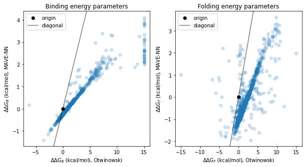
[10]:
# Set plotting routine
def draw(ax, x, y, ddG_var, title):
    ax.scatter(x, y, alpha=.2)
    xlim = ax.get_xlim()
    ax.autoscale(False)
    ax.plot(0,0,'ok', label='origin')
    ax.plot(xlim, xlim, '-k', alpha=.5, label='diagonal')
    ax.set_xlabel(f'{ddG_var} (kcal/mol), Otwinowski')
    ax.set_ylabel(f'{ddG_var} (kcal/mol), MAVE-NN')
    ax.set_title(title)
    ax.legend()

# Create figure and make plots
fig, axs = plt.subplots(1,2, figsize=(10,5))
draw(ax=axs[0],
     x=ddG_b_mat_otwinowski.ravel(),
     y=ddG_b_mat_mavenn.ravel(),
     ddG_var=r'$\Delta \Delta G_B$',
     title=r'Binding energy parameters')
draw(ax=axs[1],
     x=ddG_f_mat_otwinowski.ravel(),
     y=ddG_f_mat_mavenn.ravel(),
     ddG_var=r'$\Delta \Delta G_F$',
     title=r'Folding energy parameters')
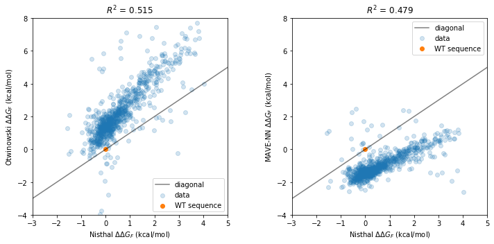
Finally, we compare our thermodynamic model’s folding energy predictions to the \(\Delta \Delta G_F\) measurements of Nisthal et al. (2019).
[11]:
# Load Nisthal data
nisthal_df = mavenn.load_example_dataset('nisthal')
nisthal_df.set_index('x', inplace=True)

# Get Nisthal folding energies relative to WT
dG_f_nisthal = nisthal_df['y']
dG_f_wt_nisthal = dG_f_nisthal[wt_seq]
ddG_f_nisthal = dG_f_nisthal - dG_f_wt_nisthal

# Get MAVE-NN folding energies relative to WT
x_nisthal = nisthal_df.index.values
x_nisthal_ohe = mavenn.src.utils.x_to_ohe(x=x_nisthal,
                                          alphabet=model.alphabet)
ddG_f_vec = ddG_f_mat_mavenn.ravel().reshape([1,-1])
ddG_f_mavenn = np.sum(ddG_f_vec*x_nisthal_ohe, axis=1)

# Get Otwinowski folding energies relative to WT
ddG_f_vec_otwinowski = ddG_f_mat_otwinowski.ravel().reshape([1,-1])
ddG_f_otwinowski = np.sum(ddG_f_vec_otwinowski*x_nisthal_ohe, axis=1)

# Define plotting routine
def draw(ax, y, model_name):
    Rsq = np.corrcoef(ddG_f_nisthal, y)[0, 1]**2
    ax.scatter(ddG_f_nisthal, y, alpha=.2, label='data')
    ax.scatter(0,0, label='WT sequence')
    xlim = [-3,5]
    ax.set_xlim(xlim)
    ax.set_ylim([-4,8])
    ax.plot(xlim, xlim, color='k', alpha=.5, label='diagonal')
    ax.set_xlabel(rf'Nisthal $\Delta \Delta G_F$ (kcal/mol)')
    ax.set_ylabel(rf'{model_name} $\Delta \Delta G_F$ (kcal/mol)')
    ax.set_title(rf'$R^2$ = {Rsq:.3f}')
    ax.legend()

# Make figure
fig, axs = plt.subplots(1,2,figsize=[10,5])
draw(ax=axs[0],
     y=ddG_f_otwinowski,
     model_name='Otwinowski')
draw(ax=axs[1],
     y=ddG_f_mavenn,
     model_name='MAVE-NN')

fig.tight_layout(w_pad=5)
References
Otwinowski J. Biophysical inference of epistasis and the effects of mutations on protein stability and function. Mol Biol Evol 35:2345–2354 (2018).
Olson CA, Wu NC, Sun R. A comprehensive biophysical description of pairwise epistasis throughout an entire protein domain. Curr Biol 24:2643–2651 (2014).
Tareen A, Posfai A, Ireland WT, McCandlish DM, Kinney JB. MAVE-NN: learning genotype-phenotype maps from multiplex assays of variant effect. bioRxiv doi:10.1101/2020.07.14.201475 (2020).
Nisthal A, Wang CY, Ary ML, Mayo SL. Protein stability engineering insights revealed by domain-wide comprehensive mutagenesis. Proc Natl Acad Sci 116:16367–16377 (2019).
[ ]: