Tutorial 5: The sort-seq E. Coli lac promoter binding analysis using a custom biophysical G-P maps

# Standard imports
import numpy as np
import pandas as pd
import matplotlib.pyplot as plt

# Special imports
import mavenn

The sort-seq MPRA data of Kinney et al., 2010. The authors in Ref. [1] used fluorescence-activated cell sorting, followed by deep sequencing, to assay gene expression levels from variant lac promoters in E. coli. The data is available in MAVE-nn load_example_dataset function and it is called 'sortseq'.

# Choose dataset
data_name = 'sortseq'

print(f"Loading dataset '{data_name}' ")

# Load datset
data_df = mavenn.load_example_dataset(data_name)

# Get and report sequence length
L = len(data_df.loc[0, 'x'])
print(f'Sequence length: {L:d} amino acids')

# Preview dataset
data_df

Loading dataset 'sortseq'
Sequence length: 75 amino acids

	set	ct_0	ct_1	ct_2	ct_3	ct_4	ct_5	ct_6	ct_7	ct_8	ct_9	x
0	training	0	1	0	0	0	0	0	0	0	0	AAAAAAAGTGAGTTAGCCAACTAATTAGGCACCGTACGCTTTATAG...
1	test	0	0	0	0	0	0	0	0	1	0	AAAAAATCTGAGTTAGCTTACTCATTAGGCACCCCAGGCTTGACAC...
2	test	0	0	0	0	0	0	1	0	0	0	AAAAAATCTGAGTTTGCTCACTCTATCGGCACCCCAGTCTTTACAC...
3	training	0	0	0	0	0	0	0	0	0	1	AAAAAATGAGAGTTAGTTCACTCATTCGGCACCACAGGCTTTACAA...
4	training	0	0	0	0	0	0	0	0	0	1	AAAAAATGGGTGTTAGCTCTATCATTAGGCACCCCCGGCTTTACAC...
...	...	...	...	...	...	...	...	...	...	...	...	...
50513	validation	0	0	0	1	0	0	0	0	0	0	TTTTGCAGAGTGTCAGCCCACTCATTACGCACCGCAGCCGTTACAC...
50514	test	0	0	0	0	0	0	0	0	1	0	TTTTTATGTGAGTTAGCTCACTCATTCGGCACCCTAGGCTTTACAC...
50515	training	0	0	0	1	0	0	0	0	0	0	TTTTTATGTGAGTTTGCTCACTCATGTGGCACCTAAGGCTTTACGC...
50516	training	1	0	0	0	0	0	0	0	0	0	TTTTTATGTGGGTTAGGTCGCGCATTAGGCACCGCAGGCTTTACCC...
50517	training	1	0	0	0	0	0	0	0	0	0	TTTTTATGTGTGTTTACTCTCTCATTAGGCACTCCACGCTTTACAC...

50518 rows × 12 columns

# Split dataset
trainval_df, test_df = mavenn.split_dataset(data_df)

# Show dataset sizes
print(f'Train + val set size : {len(trainval_df):6,d} observations')
print(f'Test set size        : {len(test_df):6,d} observations')

# Preview trainval_df
trainval_df

Training set   :   30,516 observations (  60.41%)
Validation set :   10,067 observations (  19.93%)
Test set       :    9,935 observations (  19.67%)
-------------------------------------------------
Total dataset  :   50,518 observations ( 100.00%)

Train + val set size : 40,583 observations
Test set size        :  9,935 observations

	validation	ct_0	ct_1	ct_2	ct_3	ct_4	ct_5	ct_6	ct_7	ct_8	ct_9	x
0	False	0	1	0	0	0	0	0	0	0	0	AAAAAAAGTGAGTTAGCCAACTAATTAGGCACCGTACGCTTTATAG...
1	False	0	0	0	0	0	0	0	0	0	1	AAAAAATGAGAGTTAGTTCACTCATTCGGCACCACAGGCTTTACAA...
2	False	0	0	0	0	0	0	0	0	0	1	AAAAAATGGGTGTTAGCTCTATCATTAGGCACCCCCGGCTTTACAC...
3	False	0	1	0	0	0	0	0	0	0	0	AAAAAATGTCAGTTAGCTGACTCATTAGGCACCCCTGGCTTTACGT...
4	True	0	0	0	0	0	0	1	0	0	0	AAAAAATGTGAGAAAGCTCACTCCTTTGGCACCGCAGGCTTTACAC...
...	...	...	...	...	...	...	...	...	...	...	...	...
40578	True	0	1	0	0	0	0	0	0	0	0	TTTTGATGTGGGTTTGCTCTCTCTTCAGGCACCCCACGCTTTACGC...
40579	True	0	0	0	1	0	0	0	0	0	0	TTTTGCAGAGTGTCAGCCCACTCATTACGCACCGCAGCCGTTACAC...
40580	False	0	0	0	1	0	0	0	0	0	0	TTTTTATGTGAGTTTGCTCACTCATGTGGCACCTAAGGCTTTACGC...
40581	False	1	0	0	0	0	0	0	0	0	0	TTTTTATGTGGGTTAGGTCGCGCATTAGGCACCGCAGGCTTTACCC...
40582	False	1	0	0	0	0	0	0	0	0	0	TTTTTATGTGTGTTTACTCTCTCATTAGGCACTCCACGCTTTACAC...

40583 rows × 12 columns

Training data are the count columns (10 columns) of the above dataset.

# Get the length of the sequence
L = len(data_df['x'][0])
# Get the column index for the counts
y_cols = trainval_df.columns[1:-1]
# Get the number of count columns
len_y_cols = len(y_cols)

Training

A four-state thermodynamic model for transcriptional activation at E. coli lac promoter which proposed in Ref. [1] is trained here using MAVE-NN. Here, \(\Delta G_R\) and \(\Delta G_C\) are RNAP-DNA and CRP-DNA binding Gibbs free energies and CRP-RNAP interaction energy is represented by a scalar \(\Delta G_I\). The four-state thermodynamic model is summarized below:

microstates	Gibbs free energies	activity
free DNA	0	0
CRP-DNA binding	\(\Delta G_C\)	0
RNAP-DNA binding	\(\Delta G_R\)	1
CRP and RNAP both bounded to DNA and interact	\(\Delta G_C+ \Delta G_R + \Delta G_I\)	1

The rate of transcription tr_rate has the following form:

\[tr_{\text{rate}} = t_{sat} \frac {\exp(-\Delta G_R)+ \exp(-\Delta G_C-\Delta G_R-\Delta G_I)}{1+\exp(-\Delta G_C)+ \exp(-\Delta G_R)+ \exp(-\Delta G_C- \Delta G_R- \Delta G_I)}\]

in which \(t_{sat}\) is the transcription rate resulting from full RNAP occupancy.

Here, the \(\Delta G_C\) and \(\Delta G_R\) are trainable matrices (weights of the neural network) and \(\Delta G_I\) and \(t_{sat}\) are trainable scalars.

To fit the above thermodynamic models, we used the Custom G-P maps layer implemented in 'mavenn.src.layers.gpmap'. For the detailed discussion on how to use the MAVE-NN custom G-P maps layer, checkout the thermodynamic model for IgG binding by GB1 tutorial.

from mavenn.src.layers.gpmap import GPMapLayer

# Tensorflow imports
import tensorflow as tf
import tensorflow.keras.backend as K
from tensorflow.keras.initializers import Constant

class ThermodynamicLayer(GPMapLayer):
    """
    Represents a four-stage thermodynamic model
    containing the states:
    1. free DNA
    2. CPR-DNA binding
    3. RNAP-DNA binding
    4. CPR and RNAP both bounded to DNA and interact
    """

    def __init__(self,
                 tf_start,
                 tf_end,
                 rnap_start,
                 rnap_end,
                 *args, **kwargs):
        """Construct layer instance."""

        # Call superclass
        super().__init__(*args, **kwargs)

        # set attributes
        self.tf_start = tf_start            # transcription factor starting position
        self.tf_end = tf_end                 # transcription factor ending position
        self.L_tf = tf_end - tf_start        # length of transcription factor
        self.rnap_start = rnap_start         # RNAP starting position
        self.rnap_end = rnap_end             # RNAP ending position
        self.L_rnap = rnap_end - rnap_start  # length of RNAP

        # define bias/chemical potential weight for TF/CRP energy
        self.theta_tf_0 = self.add_weight(name='theta_tf_0',
                                          shape=(1,),
                                          initializer=Constant(1.),
                                          trainable=True,
                                          regularizer=self.regularizer)

        # define bias/chemical potential weight for rnap energy
        self.theta_rnap_0 = self.add_weight(name='theta_rnap_0',
                                            shape=(1,),
                                            initializer=Constant(1.),
                                            trainable=True,
                                            regularizer=self.regularizer)

        # initialize the theta_tf
        theta_tf_shape = (1, self.L_tf, self.C)
        theta_tf_init = np.random.randn(*theta_tf_shape)/np.sqrt(self.L_tf)

        # define the weights of the layer corresponds to theta_tf
        self.theta_tf = self.add_weight(name='theta_tf',
                                        shape=theta_tf_shape,
                                        initializer=Constant(theta_tf_init),
                                        trainable=True,
                                        regularizer=self.regularizer)

        # define theta_rnap parameters
        theta_rnap_shape = (1, self.L_rnap, self.C)
        theta_rnap_init = np.random.randn(*theta_rnap_shape)/np.sqrt(self.L_rnap)

        # define the weights of the layer corresponds to theta_rnap
        self.theta_rnap = self.add_weight(name='theta_rnap',
                                          shape=theta_rnap_shape,
                                          initializer=Constant(theta_rnap_init),
                                          trainable=True,
                                          regularizer=self.regularizer)

        # define trainable real number G_I, representing interaction Gibbs energy
        self.theta_dG_I = self.add_weight(name='theta_dG_I',
                                   shape=(1,),
                                   initializer=Constant(-4),
                                   trainable=True,
                                   regularizer=self.regularizer)


    def call(self, x):
        """Process layer input and return output.

        x: (tensor)
            Input tensor that represents one-hot encoded
            sequence values.
        """

        # 1kT = 0.616 kcal/mol at body temperature
        kT = 0.616

        # extract locations of binding sites from entire lac-promoter sequence.
        # for transcription factor and rnap
        x_tf = x[:, self.C * self.tf_start:self.C * self.tf_end]
        x_rnap = x[:, self.C * self.rnap_start: self.C * self.rnap_end]

        # reshape according to tf and rnap lengths.
        x_tf = tf.reshape(x_tf, [-1, self.L_tf, self.C])
        x_rnap = tf.reshape(x_rnap, [-1, self.L_rnap, self.C])

        # compute delta G for crp binding
        G_C = self.theta_tf_0 + \
            tf.reshape(K.sum(self.theta_tf * x_tf, axis=[1, 2]),
                       shape=[-1, 1])

        # compute delta G for rnap binding
        G_R = self.theta_rnap_0 + \
            tf.reshape(K.sum(self.theta_rnap * x_rnap, axis=[1, 2]),
                       shape=[-1, 1])

        G_I = self.theta_dG_I

        # compute phi
        numerator_of_rate = K.exp(-G_R/kT) + K.exp(-(G_C+G_R+G_I)/kT)
        denom_of_rate = 1.0 + K.exp(-G_C/kT) + K.exp(-G_R/kT) + K.exp(-(G_C+G_R+G_I)/kT)
        phi = numerator_of_rate/denom_of_rate

        return phi

Training the Model

Here we train the model with MAVEN. Note that we initialize the Gibbs energies with random negative values to help the convergence of the training.

# define custom gp_map parameters dictionary
gpmap_kwargs = {'tf_start': 1,  # starting position of the CRP
                'tf_end': 27,  # ending position of the CRP
                'rnap_start': 34,  # starting position of the RNAP
                'rnap_end': 75,   # ending position of the RNAP
                'L': L,
                'C': 4,
                'theta_regularization': 0.1}

# Create model
model = mavenn.Model(L=L,
                     Y=len_y_cols,
                     alphabet='dna',
                     regression_type='MPA',
                     gpmap_type='custom',
                     gpmap_kwargs=gpmap_kwargs,
                     custom_gpmap=ThermodynamicLayer);

# Set training data
model.set_data(x=trainval_df['x'],
               y=trainval_df[y_cols],
               validation_flags=trainval_df['validation'],
               shuffle=True);

# Fit model to data
model.fit(learning_rate=5e-4,
          epochs=2000,
          batch_size=100,
          early_stopping=True,
          early_stopping_patience=25,
          linear_initialization=False,
          verbose=False);

N = 40,583 observations set as training data.
Using 24.8% for validation.
Data shuffled.
Time to set data: 0.447 sec.

Training time: 71.6 seconds

model.save('sortseq_thermodynamic_mpa')

Model saved to these files:
        sortseq_thermodynamic_mpa.pickle
        sortseq_thermodynamic_mpa.h5

# Compute predictive information on test data
I_pred, dI_pred = model.I_predictive(x=test_df['x'], y=test_df[y_cols])
print(f'test_I_pred: {I_pred:.3f} +- {dI_pred:.3f} bits')

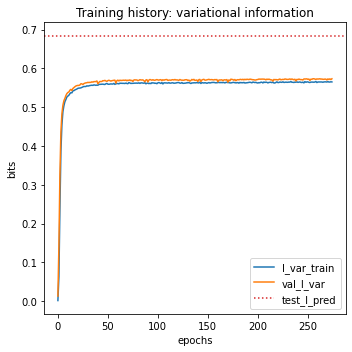
test_I_pred: 0.685 +- 0.011 bits

# Create figure and axes for plotting
fig, ax = plt.subplots(1, 1, figsize=[5, 5])

# Plot I_var_train, the variational information on training data as a function of epoch
ax.plot(model.history['I_var'], label=r'I_var_train')

# Plot I_var_val, the variational information on validation data as a function of epoch
ax.plot(model.history['val_I_var'], label=r'val_I_var')

# Show I_pred_test, the predictive information of the final model on test data
ax.axhline(I_pred, color='C3', linestyle=':', label=r'test_I_pred')

# Style plot
ax.set_xlabel('epochs')
ax.set_ylabel('bits')
ax.set_title('Training history: variational information')
ax.legend()

plt.tight_layout()

# Get the trained model parameters
# Retrieve G-P map parameter dict and view dict keys
param_dict = model.layer_gpmap.get_params()
param_dict.keys()

dict_keys(['theta_tf_0', 'theta_rnap_0', 'theta_tf', 'theta_rnap', 'theta_dG_I'])

Authors in Ref. [1], reported they inferred CRP-RNAP interaction energy to be \(\Delta G_I = −3.26\) kcal∕mol. The MAVE-NN prediction is very similar to the reported value, while it is several order of magnitude faster than the method used in Ref. [1].

delta_G_I = param_dict['theta_dG_I']  # Gibbs energy of Interaction (scalar)
print(f'CRP-RNAP interaction energy = {delta_G_I*0.62:.3f} k_cal/mol')

CRP-RNAP interaction energy = -1.549 k_cal/mol

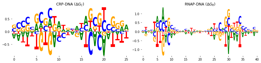
In addition, we can represent the CRP-DNA \(\Delta G_C\) and RNAP-DNA \(\Delta G_R\) binding energies in the weight matrix form. The weight matrices can be represented by sequence logos. To do that, we used the a Python package Logomaker which is also developed in our research group and is freely available here. To represent the weight matrices in logo

1. we get the trained crp_weights and rnap_weights values,

2. we convert them to the pandas.DataFrame with column names being the nucleotide strings.

The pandas.DataFrame can easily imported in Logomaker. See the documentation of Logomaker for detailed description of the parameters one can pass to make logos.

# import logomaker
import logomaker

# Get the \Delta G_C trained values (theta_tf)
crp_weights = param_dict['theta_tf']
# Get the \Delta G_R trained values (theta_rnap)
rnap_weights = param_dict['theta_rnap']
# Convert them to pandas dataframe
crp_df = pd.DataFrame(crp_weights, columns=model.alphabet)
rnap_df = pd.DataFrame(rnap_weights, columns=model.alphabet)


# plot logos
fig, axs = plt.subplots(1, 2, figsize=[12, 3])

# sequence logo for the CRP-DNA binding energy matrix
logo = logomaker.Logo(crp_df,  ax=axs[0], center_values=True)
axs[0].set_title('CRP-DNA ($\Delta G_C$)')
logo.style_spines(visible=False)


# sequence logo for the RNAP-DNA binding energy matrix
logo = logomaker.Logo(rnap_df, ax=axs[1], center_values=True)
axs[1].set_title('RNAP-DNA ($\Delta G_R$)')
logo.style_spines(visible=False)

plt.tight_layout()

References

1. Kinney J, Murugan A, Callan C, Cox E (2010). Using deep sequencing to characterize the biophysical mechanism of a transcriptional regulatory sequence. Proc Natl Acad Sci USA. 107(20):9158-9163.